Activation Functions

There’s a famous result in neural networks called the Universal Approximation Theorem. It says that a feedforward network with even a single hidden layer can approximate any continuous function — as long as it uses non-linear activation functions and has enough neurons.

The reason is simple.

If you only stack linear transformations,

\[y = w_4(w_3(w_2(w_1 x)))\]

you still end up with a linear function. Depth doesn’t help — you can only learn linear decision boundaries. Real problems are rarely linear. Non-linear activations are what give neural networks their expressive power.

---

Sigmoid — where it all started (and why we moved on)

The sigmoid function

\[\sigma(x) = \frac{1}{1 + e^{-x}}\]

was the default choice in early neural networks. It maps everything neatly into $(0,1)$, and its derivative has a clean form:

\[\sigma'(x) = \sigma(x)(1 - \sigma(x))\]

But sigmoid comes with serious drawbacks.

Vanishing gradients

When the output approaches 0 or 1, the neuron saturates and the derivative goes to zero. During backpropagation, gradients shrink as they move backward through layers. In deep networks this effectively kills learning — weights stop updating and training stalls.

Think about it: if $\sigma(x) = 0.99$, then
$\sigma’(x) = 0.99 \times 0.01 = 0.0099$. That’s a tiny gradient. Now multiply this across 10 layers and you get essentially zero. Your network can’t learn.

Not zero-centered

Sigmoid outputs are always positive (between 0 and 1). This creates a subtle but important problem during optimization.

Consider a neuron receiving two inputs $h_{21}$ and $h_{22}$ (both positive because they come from sigmoid activations). The gradients for weights are:

\[\nabla w_1 = \frac{\partial L}{\partial y} \cdot \frac{\partial y}{\partial h_3} \cdot \frac{\partial h_3}{\partial a_3} \cdot h_{21}\] \[\nabla w_2 = \frac{\partial L}{\partial y} \cdot \frac{\partial y}{\partial h_3} \cdot \frac{\partial h_3}{\partial a_3} \cdot h_{22}\]

Notice that if the first part (the common terms in red) is positive, both $\nabla w_1$ and $\nabla w_2$ must be positive because $h_{21}$ and $h_{22}$ are positive. If it’s negative, both gradients are negative.

This means gradient descent can only move in certain directions in weight space — not diagonally. You’re forced to zig-zag toward the optimum, which is inefficient.

Computational cost

Computing exponentials millions of times per training step isn’t cheap — especially compared to simpler activations.

For all these reasons, sigmoid is now mostly avoided in hidden layers.

---

Tanh — a small improvement

Tanh fixes one issue: it is zero-centered, mapping inputs to $(-1, 1)$. That helps optimization.

\[\tanh(x) = \frac{e^x - e^{-x}}{e^x + e^{-x}}\]

Derivative:

\[\frac{d}{dx}\tanh(x) = 1 - \tanh^2(x)\]

But it still suffers from saturation, vanishing gradients, and expensive exponential computation. So while better than sigmoid, it doesn’t solve the core training problems in deep networks.

---

ReLU — the breakthrough

Then came the simplest idea:

\[f(x) = \max(0, x)\]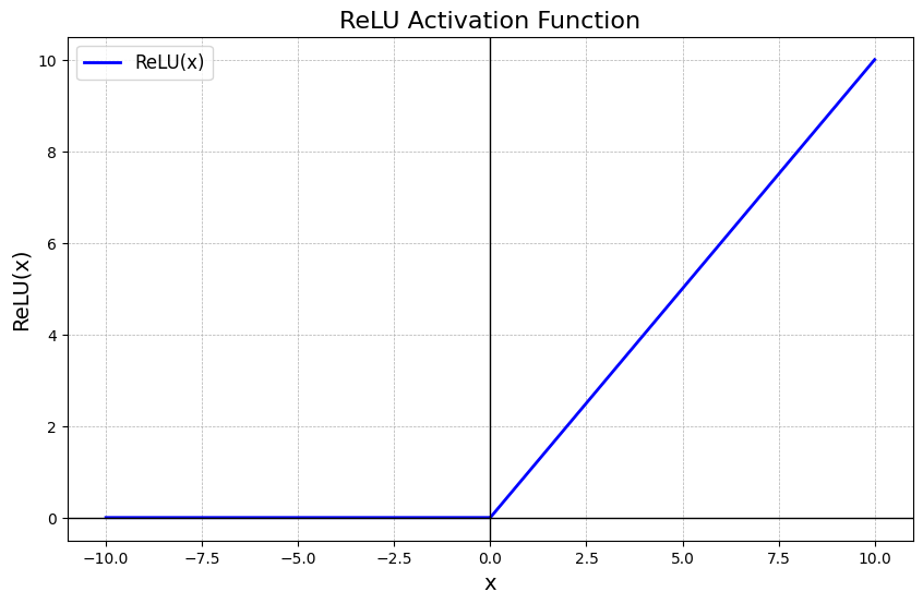

ReLU changed everything.

No saturation for positive values → gradients flow cleanly. Extremely cheap to compute (just a comparison). In practice, networks train 6x faster than with sigmoid or tanh on datasets like ImageNet.

ReLU made deep learning practical at scale.

The downside: dying neurons

Here’s the problem: if a large gradient update pushes the bias to a big negative value, the pre-activation $w_1x_1 + w_2x_2 + b$ becomes negative. The neuron outputs 0.

But here’s the worse part — the gradient $\frac{\partial h_1}{\partial a_1}$ is also 0. So when you compute:

\[\nabla w_1 = \frac{\partial L}{\partial y} \cdot \frac{\partial y}{\partial a_2} \cdot \frac{\partial a_2}{\partial h_1} \cdot \frac{\partial h_1}{\partial a_1} \cdot \frac{\partial a_1}{\partial w_1}\]

That zero term means the weights never update again. The neuron stays dead forever.

Solutions:

• Initialize biases to small positive values (like 0.01)
• Use careful learning rates
• Try ReLU variants

In practice, a large fraction of ReLU neurons can die if you set the learning rate too high.

---

ReLU variants that fix dying neurons

Leaky ReLU

\[f(x) = \max(\alpha x, x), \quad \alpha \approx 0.01\]

Keeps a small gradient alive for negative inputs. The $0.01x$ ensures at least some signal flows backward.

Parametric ReLU (PReLU)

Same idea, but $\alpha$ is learned during training. Let the network figure out the best slope.

ELU (Exponential Linear Unit)

\[f(x) = \begin{cases} x & x > 0 \\ \alpha(e^x - 1) & x \le 0 \end{cases}\]

Produces negative outputs, making activations closer to zero-centered. The exponential term ensures gradients flow smoothly even for negative values. Downside: computing $e^x$ is expensive.

Maxout

\[f(x) = \max(w_1x + b_1, \dots, w_kx + b_k)\]

Generalizes both ReLU and Leaky ReLU. For example:

• $\max(0.5x, -0.5x)$ gives you absolute value
• $\max(0, w_2^Tx + b_2)$ is just ReLU

No saturation, no death. Two Maxout neurons can even act as a universal approximator. But you pay with k× more parameters.

---

Modern activations: GELU, SELU, Swish

GELU (Gaussian Error Linear Unit)

ReLU multiplies input by either 1 or 0 based on sign. Dropout also randomly multiplies by 1 or 0. GELU combines these ideas.

Instead of a hard cutoff, GELU weights inputs probabilistically using the cumulative distribution function of a standard normal distribution:

\[\text{GELU}(x) = x \cdot P(X \le x), \quad X \sim \mathcal{N}(0,1)\]

The idea: let the multiplication factor be random and depend on the input. The range needs to be between 0 and 1, so the natural choice is the CDF of a Gaussian.

In practice, it’s approximated as:

\[\text{GELU}(x) \approx 0.5x\left(1 + \tanh\left[\sqrt{\frac{2}{\pi}}(x + 0.044715x^3)\right]\right)\]

or more simply:

\[\text{GELU}(x) \approx x \cdot \sigma(1.702x)\]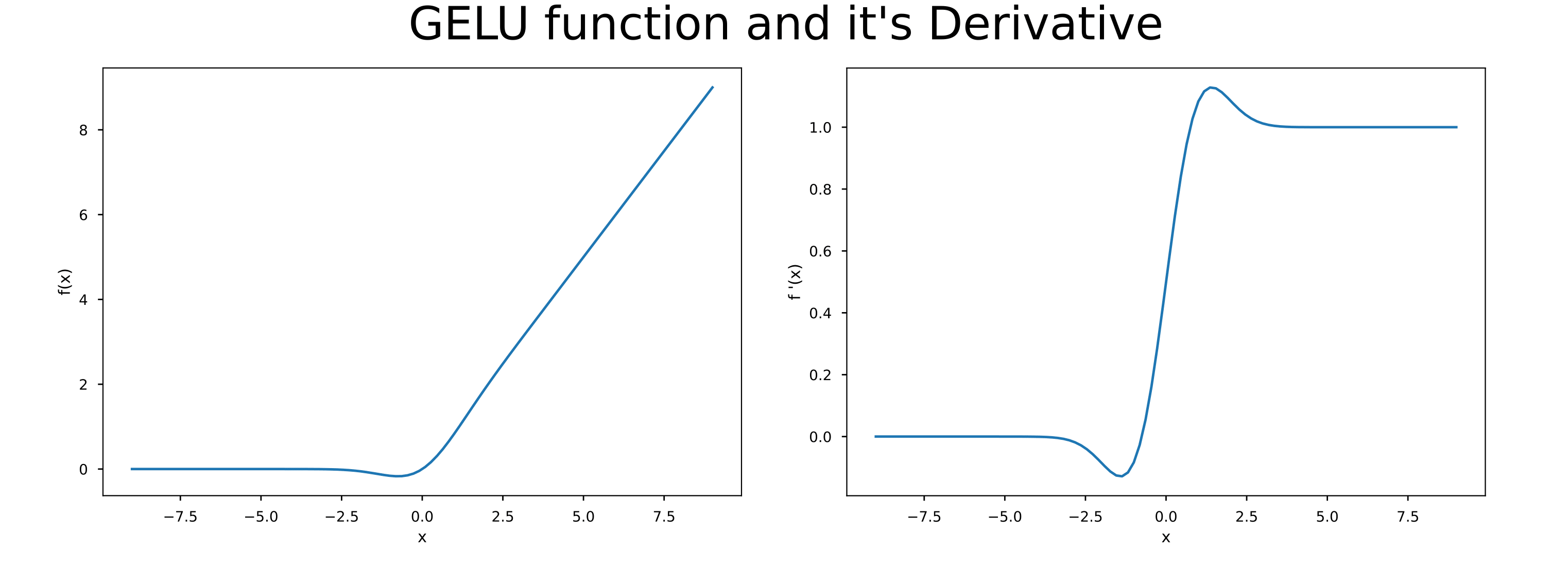

GELU is now the standard activation in transformers — used in BERT, GPT, and most modern language models.

---

SELU (Scaled Exponential Linear Unit)

SELU is designed to be self-normalizing. Ideally, you want activations from each layer to have zero mean and unit variance. Normally you’d use batch normalization for this. SELU does it automatically.

\[f(x) = \lambda \begin{cases} x & x > 0 \\ \alpha(e^x - 1) & x \le 0 \end{cases}\]

With carefully chosen constants $\lambda \approx 1.0507$ and
$\alpha \approx 1.6733$, activations naturally maintain zero mean and unit variance across layers , often removing the need for batch normalization.

---

Swish / SiLU (Sigmoid-weighted Linear Unit)

Researchers used automated search methods (basically letting algorithms search through possible activation functions) and discovered:

\[f(x) = x \cdot \sigma(\beta x)\]

When $\beta = 1$, it’s called SiLU. When $\beta$ is learnable, it’s Swish.

Interestingly, this was actually proposed earlier in the reinforcement learning community, but the search methods rediscovered it. It often outperforms ReLU in deep networks and is widely used in modern CNNs.

---

What actually works in practice

CNNs → ReLU or Swish/SiLU (ReLU is still the standard, works well, fast)

Transformers / NLP → GELU (the default for BERT, GPT, and modern language models)

RNN gates → Sigmoid and tanh (still useful specifically for gating mechanisms in LSTMs)

Deep fully connected nets → Leaky ReLU, ELU, or GELU

Avoid sigmoid in hidden layers unless you have a very specific reason. The vanishing gradient problem is real.

---